Ornaments

Ornaments designate all the extra elements you can add to a figure to beautify it or to make it clearer. Ornaments include standard elements such as legend, annotation, colorbars, text but you can also design your own element specifically for your figure. For example, figure figure-bessel-functions displays a mix of standard elements (annotation and text) as well as specific elements (roots reported on the x axis using vertical markers).

Bessel functions figure-bessel-functions (sources: ornaments/bessel-functions.py).

There is no theoretical limit in the number of ornaments you can add to a figure. However, you have to take care that your figure is still easily readable and not too overloaded.

Legend

Legends are quite easy to use and only require for the user to name plots. Matplotlib will take care of placing the legend automatically (which is really tricky and consequently it can fail) and display the necessary information (see figure figure-legend-regular). Legend comes with several options that allows you to control every aspect of the legend even if, most of the time, a simple legend() call is sufficient as shown below:

fig = plt.figure(figsize=(6,2.5))
ax = plt.subplot()

X = np.linspace(-np.pi, np.pi, 256, endpoint=True)
ax.plot(X, np.cos(X), label="cosine")
ax.plot(X, np.sin(X), label="sine")
ax.legend()

plt.show()

Regular legend figure-legend-regular (sources: ornaments/legend-regular.py).

Alternative legends figure-legend-alternatives (sources: ornaments/legend-alternatives.py).

However, there are some cases where legend might not be the most appropriate way to add information. For example, when you have several plots, it may become tedious for the reader to go back and forth between plots and legend. An alternative way is to add information directly on the plots as shown on figure figure-legend-alternatives.

This figure introduces four different ways to directly label plots even though there is no best alternative because it really depends on the data. For the displayed sine / cosine example (which is quite simple) the four solutions are appropriate, but when used with real data, it may happen that none of these alternative suits the data. In such case, you might need an alternate way of labelling data or you may need to split your figure into several plots.

Title & labels

We’ve already manipulated title and labels using set_title, set_xlabel and set_ylabel methods. When used without any extra argument, they do a fairly good job and their placement is usually good for most figures. Nonetheless, it is possible to play with the various parameters such as to beautify the figure as shown on figure figure-title-regular. In this example, I simply displaced the labels in order to be closer to the axis and I took care of removing the central tick that would have else collided with the label. For the title, I simply moved it to the right and I moved the legend box (using two columns) accordingly, that is, under the title. Nothing complicated here but I think the result is visually more pleasant.

Regular title figure-title-regular (sources: ornaments/title-regular.py).

In some cases (e.g. conference poster), you may need to have titles to be a little more eye catching like shown on figure figure-latex-text-box. This is made possible by dividing each axis with the make_axes_locatable method and to reserve 15% of height for the actual title. In this figure, I also inserted a fully justified text using Latex that may be considered as another form or (advanced) ornament.

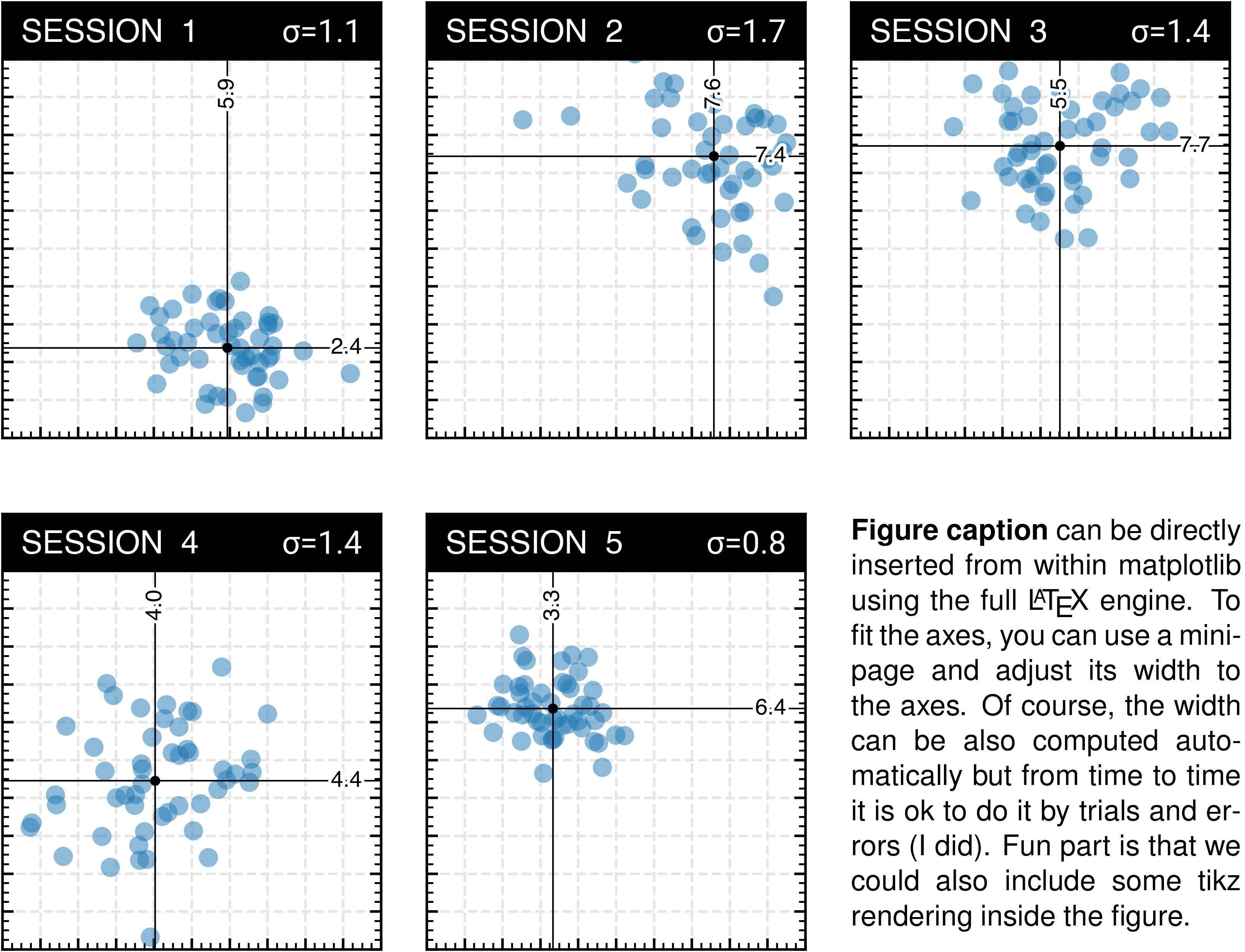
Advanced text box figure-latex-text-box (sources: ornaments/latex-text-box.py).

Annotations

Annotation is probably the most difficult object to handle inside matplotlib. The reason is that it involves a number of different concepts that results in a potential high number of parameters. Furthermore, there is a supplementary difficulty because annotation involve text whose size is expressed in points. In the end, you may have to mix absolute or relative coordinates in pixels, points, fractions or data units. If you add the fact that you can annotate any axis having any kind of projection, you may now realize why the annotate method offer so many parameters.

The simplest way to annotate a figure is to add labels very close to the points you want to annotate as shown on figure figure-annotation-direct. In this figure, I took care of adding a white outline to the labels such that they remain readable, independently of the data distribution. However, if you have too many points, all the different labels may end up cluttering your figure and hide potentially important information.

Direct annotations figure-annotation-direct (sources: ornaments/annotation-direct.py).

An alternative is to push labels on the side of the figure and to use broken lines to establish the link between the point and the label as shown on figure figure-annotation-side. But this is far from being automatic and to design this figure, I had to compute pretty much everything. First, to have lines to not cross each other, I order the point I want to label:

X = np.random.normal(0, .35, 1000)
Y = np.random.normal(0, .35, 1000)
ax.scatter(X, Y, edgecolor="None", facecolor="C1", alpha=0.5)

I = np.random.choice(len(X), size=5, replace=False)
Px, Py = X[I], Y[I]
I = np.argsort(Y[I])[::-1]
Px, Py = Px[I], Py[I]

From these points, I’ve been able to annotate them using a quite complex connection style:

y, dy = .25, 0.125
style = "arc,angleA=-0,angleB=0,armA=-100,armB=0,rad=0"
for i in range(len(I)):
    ax.annotate("Point " + chr(ord("A")+i),
                xy = (Px[i], Py[i]),    xycoords='data',
                xytext = (1.25, y-i*dy),  textcoords='data',
                arrowprops=dict(arrowstyle="->", color="black",
                                linewidth=.75,
                                shrinkA=20, shrinkB=5,
                                patchA=None, patchB=None,
                                connectionstyle=style))

Side annotations figure-annotation-side (sources: ornaments/annotation-side.py).

It is also possible to annotate objects outside the axes using a connection patch as shown on figure figure-annotation-zoom. In this example, I created several rectangles showing areas of interest around some points and I created a connection to the corresponding zoomed axes. Note how the connection starts on the outside of the rectangle, which is one of the nice feature offered by annotation: you can specify the nature of the object you want to annotate (by providing a patch) and matplotlib will take care of having the origin of the connection to the border of the patch.

Zoomed annotations figure-annotation-zoom (sources: ornaments/annotation-zoom.py).

Exercise

It is now your turn to experiment with ornaments by trying to reproduce the figure figure-elegant-scatter which displays several ornaments, including a custom one on the left and bottom side. This ornament provides a quick way to show respective distributions along weight and height and can be rendered with a scatter plot using large vertical and horizontal markers.

Elegant scatter plot figure-elegant-scatter (sources: ornaments/elegant-scatter.py).