Mastering the defaults

We’ve just explained (see rule 5 in chapter chap-rules_) that any visualization library or software comes with a set of default settings that identifies it. For example, figure figure-sine-cosine-variants show the sine and cosine functions as rendered by Google calculator, Julia, Gnuplot and Matlab. Even for such simple functions, these displays are quite characteristic.

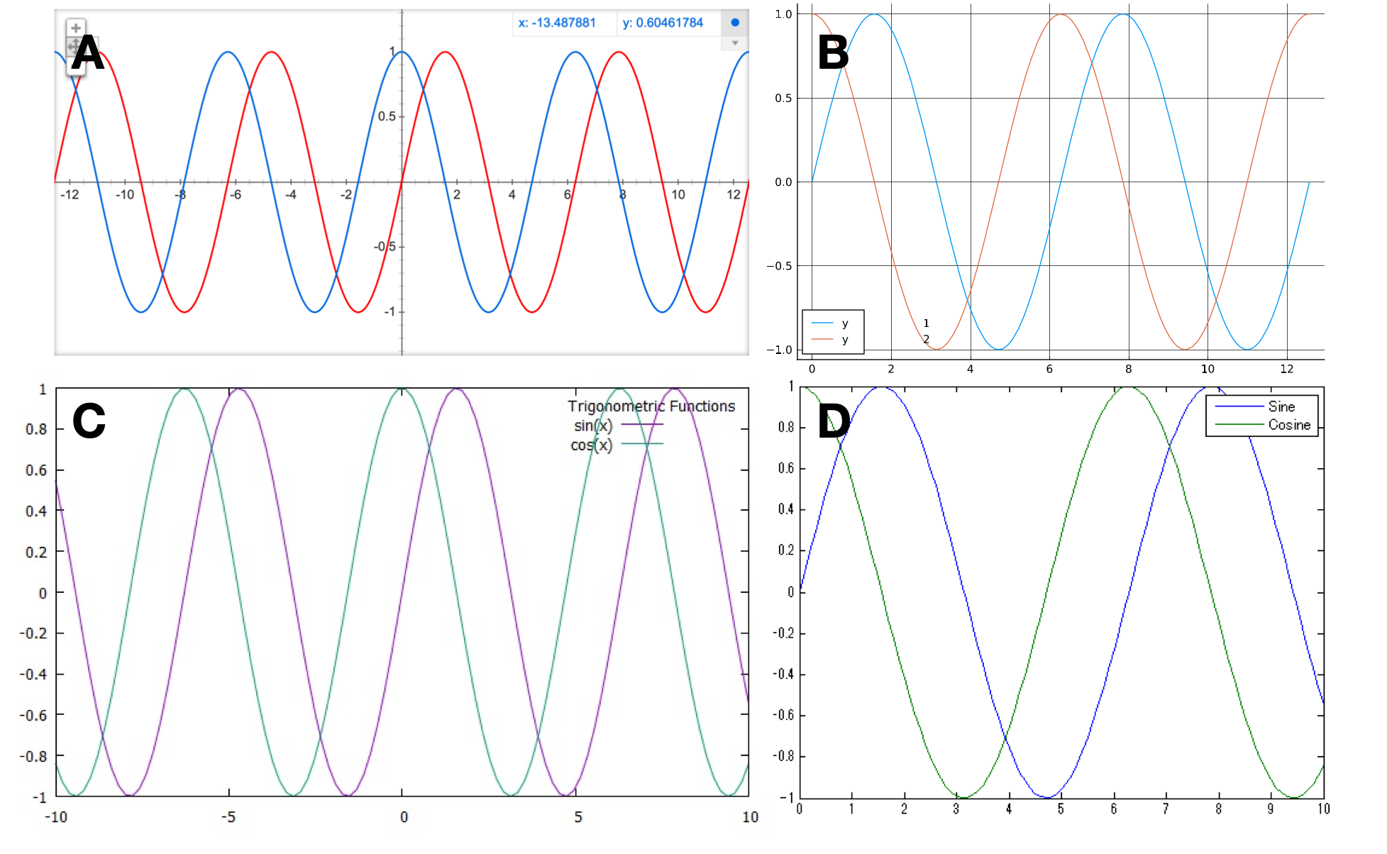
Sine and cosine functions as displayed by (A) Google calculator (B) Julia, (C) Gnuplot (D) Matlab. figure-sine-cosine-variants

Let’s draw sine and cosine functions using Matplotlib defaults.

import numpy as np
import matplotlib.pyplot as plt

X = np.linspace(-np.pi, np.pi, 256, endpoint=True)
C, S = np.cos(X), np.sin(X)
plt.plot(X, C)
plt.plot(X, S)
plt.show()

Figure figure-defaults-step-2 shows the result that is quite characteristic of Matplotlib.

Sine and cosine functions with implicit defaults (sources defaults/defaults-step-1.py) figure-defaults-step-1

Explicit settings

Let’s now redo the figure but with the specification of all the different settings. This includes, figure size, line colors, widths and styles, ticks positions and labels, axes limits, etc.

fig = plt.figure(figsize = p['figure.figsize'],
                 dpi = p['figure.dpi'],
                 facecolor = p['figure.facecolor'],
                 edgecolor = p['figure.edgecolor'],
                 frameon = p['figure.frameon'])
ax = plt.subplot(1,1,1)

ax.plot(X, C, color="C0",
              linewidth = p['lines.linewidth'],
              linestyle = p['lines.linestyle'])
ax.plot(X, S, color="C1",
              linewidth = p['lines.linewidth'],
              linestyle = p['lines.linestyle'])

xmin, xmax = X.min(), X.max()
xmargin = p['axes.xmargin']*(xmax - xmin)
ax.set_xlim(xmin - xmargin, xmax + xmargin)

ymin, ymax = min(C.min(), S.min()), max(C.max(), S.max())
ymargin = p['axes.ymargin']*(ymax - ymin)
ax.set_ylim(ymin - ymargin, ymax + ymargin)

ax.tick_params(axis = "x", which="major",
               direction = p['xtick.direction'],
               length = p['xtick.major.size'],
               width = p['xtick.major.width'])
ax.tick_params(axis = "y", which="major",
               direction = p['ytick.direction'],
               length = p['ytick.major.size'],
               width = p['ytick.major.width'])
plt.show()

Sine and cosine functions using matplotlib explicit defaults (sources defaults/defaults-step-2.py) figure-defaults-step-2

The resulting figure figure-defaults-step-2 is an exact copy of figure-defaults-step-1. This comes as no surprise because I took care of reading the default values that are used implicitly by Matplotlib and set them explicitly. In fact, there are many more default choices that I did not materialize in this short example. For instance, the font family, slant, weight and size of tick labels can be configured in the defaults.

User settings

Note that we can also do the opposite and change the defaults before creating the figure. This way, matplotlib will use our custom defaults instead of standard ones. The result is shown on figure figure-defaults-step-3 where I changed a number of settings. Unfortunately, not every settings can be modified this way. For example, the position of markers (markevery) cannot yet be set.

p["figure.figsize"] = 6,2.5
p["figure.edgecolor"] = "black"
p["figure.facecolor"] = "#f9f9f9"

p["axes.linewidth"] = 1
p["axes.facecolor"] = "#f9f9f9"
p["axes.ymargin"] = 0.1
p["axes.spines.bottom"] = True
p["axes.spines.left"] = True
p["axes.spines.right"] = False
p["axes.spines.top"] = False
p["font.sans-serif"] = ["Fira Sans Condensed"]

p["axes.grid"] = False
p["grid.color"] = "black"
p["grid.linewidth"] = .1

p["xtick.bottom"] = True
p["xtick.top"] = False
p["xtick.direction"] = "out"
p["xtick.major.size"] = 5
p["xtick.major.width"] = 1
p["xtick.minor.size"] = 3
p["xtick.minor.width"] = .5
p["xtick.minor.visible"] = True

p["ytick.left"] = True
p["ytick.right"] = False
p["ytick.direction"] = "out"
p["ytick.major.size"] = 5
p["ytick.major.width"] = 1
p["ytick.minor.size"] = 3
p["ytick.minor.width"] = .5
p["ytick.minor.visible"] = True

p["lines.linewidth"] = 2
p["lines.markersize"] = 5

fig = plt.figure(linewidth=1)
ax = plt.subplot(1,1,1,aspect=1)
ax.plot(X, C)
ax.plot(X, S)

plt.show()

Sine and cosine functions using custom defaults (sources defaults/defaults-step-3.py) figure-defaults-step-3

Stylesheets

Changing default settings is thus an easy way to customize the style of your figure. But writing such style inside the figure script as we did until now is not very convenient and this is where style comes into play. Styles are small text files describing (some) settings in the same way as they are defined in the main resource file matplotlibrc:

figure.figsize: 6,2.5
figure.edgecolor: black
figure.facecolor: ffffff

axes.linewidth: 1
axes.facecolor: ffffff
axes.ymargin: 0.1
axes.spines.bottom: True
axes.spines.left: True
axes.spines.right: False
axes.spines.top: False
font.sans-serif: Fira Sans Condensed

axes.grid: False
grid.color: black
grid.linewidth: .1

xtick.bottom: True
xtick.top: False
xtick.direction: out
xtick.major.size: 5
xtick.major.width: 1
xtick.minor.size: 3
xtick.minor.width: .5
xtick.minor.visible: True

ytick.left: True
ytick.right: False
ytick.direction: out
ytick.major.size: 5
ytick.major.width: 1
ytick.minor.size: 3
ytick.minor.width: .5
ytick.minor.visible: True

lines.linewidth: 2
lines.markersize: 5

And we can now write:

plt.style.use("./mystyle.txt")

fig = plt.figure(linewidth=1)
ax = plt.subplot(1,1,1,aspect=1)
ax.plot(X, C)
ax.plot(X, S)
ax.set_yticks([-1,0,1])

Beyond stylesheets

If stylesheet allows to set a fair number of parameters, there is still plenty of other things that can be changed to improve the style of a figure even though we cannot use the stylesheet to do so. One of the reason is that these settings are specific to a given figure and it wouldn’t make sense to set them in the stylesheet. In the sine and cosine case, we can for example specify explicitly the location and labels of xticks, taking advantage of the fact that we know that we’re dealing with trigonometry functions:

ax.set_yticks([-1,1])
ax.set_yticklabels(["-1", "+1"])

ax.set_xticks([-np.pi, -np.pi/2, np.pi/2, np.pi])
ax.set_xticklabels(["-π", "-π/2", "+π/2", "+π"])

We can also move the spines such as to center them:

ax.spines['bottom'].set_position(('data',0))
ax.spines['left'].set_position(('data',0))

And add some arrows at axis ends:

ax.plot(1, 0, ">k",
        transform=ax.get_yaxis_transform(), clip_on=False)
ax.plot(0, 1, "^k",
        transform=ax.get_xaxis_transform(), clip_on=False)

You can see the result on figure figure-defaults-step-5. From this, you can start refining further the figure. But remember that if it’s ok to tweak parameters a bit, you can also lose a lot of time doing that (trust me).

Sine and cosine functions using custom defaults and fine tuning. (sources defaults/defaults-step-5.py) figure-defaults-step-5

Exercise

Starting from the code below try to reproduce figure figure-defaults-exercise-1 by modifying only rc settings.

fig = plt.figure()
ax = plt.subplot(1,1,1,aspect=1)
ax.plot(X, C, markevery=(0, 64), clip_on=False, zorder=10)
ax.plot(X, S, markevery=(0, 64), clip_on=False, zorder=10)
ax.set_yticks([-1,0,1])
ax.set_xticks([-np.pi, -np.pi/2, 0, np.pi/2, np.pi])
ax.set_xticklabels(["-π", "-π/2", "0", "+π/2", "+π"])
ax.spines['bottom'].set_position(('data',0))

Alternative rendering of sine and cosine (solution defaults/defaults-exercice-1.py) figure-defaults-exercise-1