Architecture & optimization

Even though a deep understanding of the matplotlib architecture is not necessary to use it, it is nonetheless useful to know a bit of its architecture to optimize either speed, memory and even rendering.

Transparency levels

We’ve already seen how to use transparency in a scatter plot to have a perception of data density. This works reasonably well if you don’t have too much data. But what is too much exactly? It would be hard to give a definitive limit because it depends on a number of parameters such as the size of your figure, the shape and size of your markers and the alpha level (i.e. transparency). For this latter, there is actually a limit in how much transparent a color can be and it is exactly 0.002 (= 1/500). This means that if you plot 500 black points with a transparency of 0.002, you obtain get a quasi black marker as shown on figure figure-transparency.

Transparency levels figure-transparency (sources: optimization/transparency.py).

It is not exactly black for 500 points because it also depends on how alpha compositing is computed internally but it provides nonetheless a useful approximation. Knowing this limit exists, it explains why you get a solid color in dense areas when you have a lot of data. This is illustrated on figure figure-scatters where the number of data is respectively 10,000, 100,000 and 1,000,000. For 10,000 and 100,000 points we can adapt the transparency level to show where are the dense areas. In this case, this is simple normal distribution and we can observe the central are is darker. For one million points, we reached the limit of the transparency trick (alpha=0.002) and we now have a central dark spot that hide information.

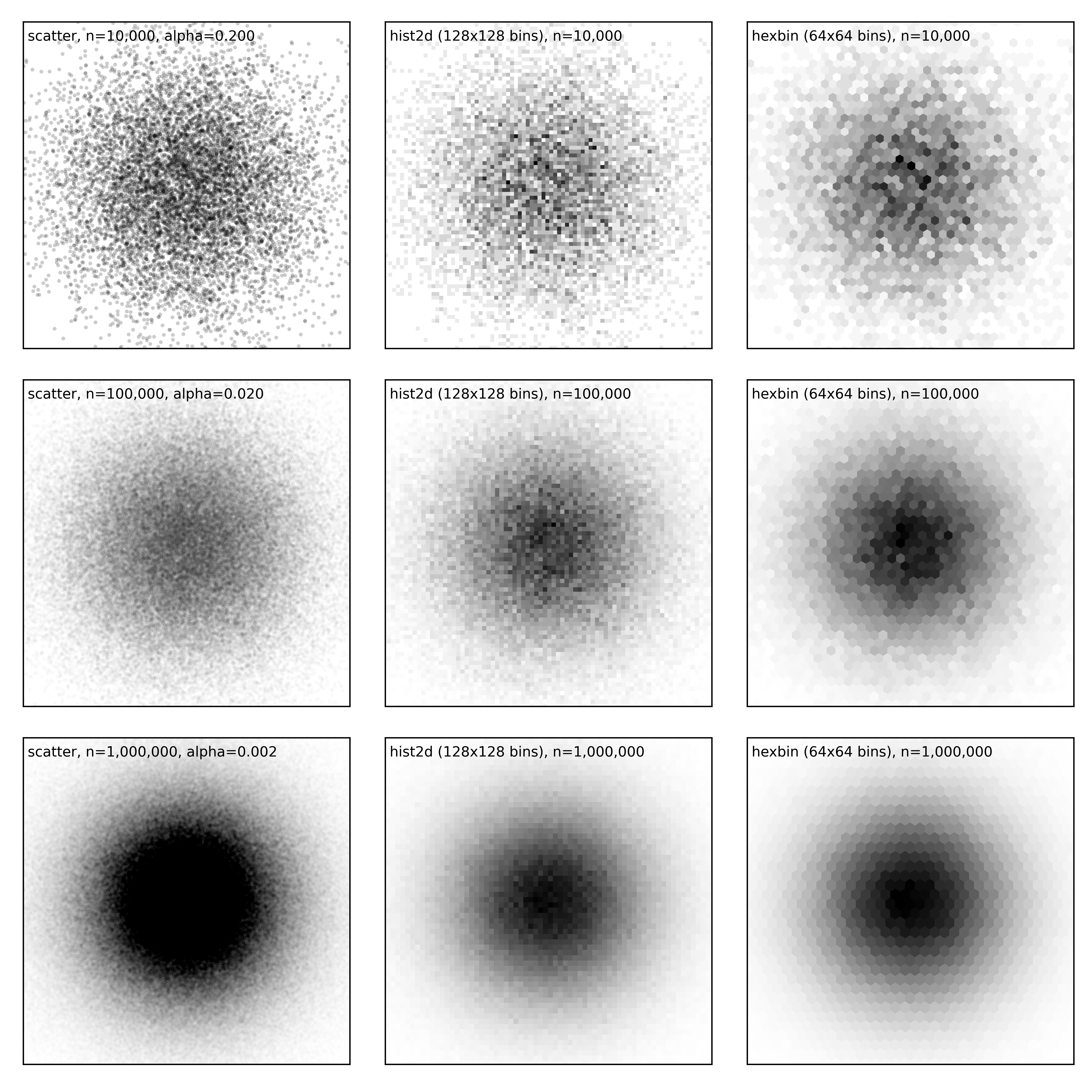
Scatter, hist2d and hexbin figure-scatters (sources: optimization/scatters.py).

This means we need a new strategy to display the data. Fortunately, matplotlib provides hist2d and hexbin that will both aggregate points into bins (with square or hex shape) that are eventually colored according to the number in the bins. This allows to visualize density for any number of data points and do not require to manipulate size and/or transparency of markers. You’re now ready to reproduce Todd W. Schneider’s astonishing visualization of NYC Taxi trips (Analyzing 1.1 Billion NYC Taxi and Uber Trips, with a Vengeance).

Alpha compositing induces other kind of problems with line plots, especially when a plot is self-covering itself as exemplified of a a high-frequency signal shown on figure figure-multisample. The signal is a product of two sine waves of different frequency and reads:

xmin, xmax = 0*np.pi, 5*np.pi
ymin, ymax = -1.1, +1.1
def f(x): return np.sin(np.power(x,3)) * np.sin(x)
X = np.linspace(xmin,xmax,10000)
Y = f(X)

When we plot this signal, we can see that the density of lines becomes higher and higher from left to right. Near the right side of the plot, the frequency is the highest and is actually higher than the screen resolution such that there is no empty spaces between successive waves. However, when we use a regular plot (first line of figure figure-multisample) with some transparency, we do not see a change in color (while we could expect the plot to self-cover itself). The reason is that matplotlib rendering engine takes care of not overdrawing an area that belong to the same plot as shown on the figure below:

Self-covering example figure-self-cover (sources: optimization/self-cover.py).

This explains why we do not have color change in figure figure-multisample. To counter this effect, we can render the same plot using a line collection made of individual segments. In such case, each segment is considered separately and will influence other segments. This corresponds to the second line on the figure and now we can observe a change in the color with darker colors on the right suggesting a higher frequency.

We can also adopt a totally different strategy by multisampling the signal, which is a standard techniques in signal processing. Instead of plotting the signal, I created an empty image with enough resolution and for each point (pixel) of this image, I considered 8 samples point randomly but closely distributed around the point to decide of its value. This is of course a slower compared to a regular plot but the rendering is more faithful to the signal as shown on the third line.

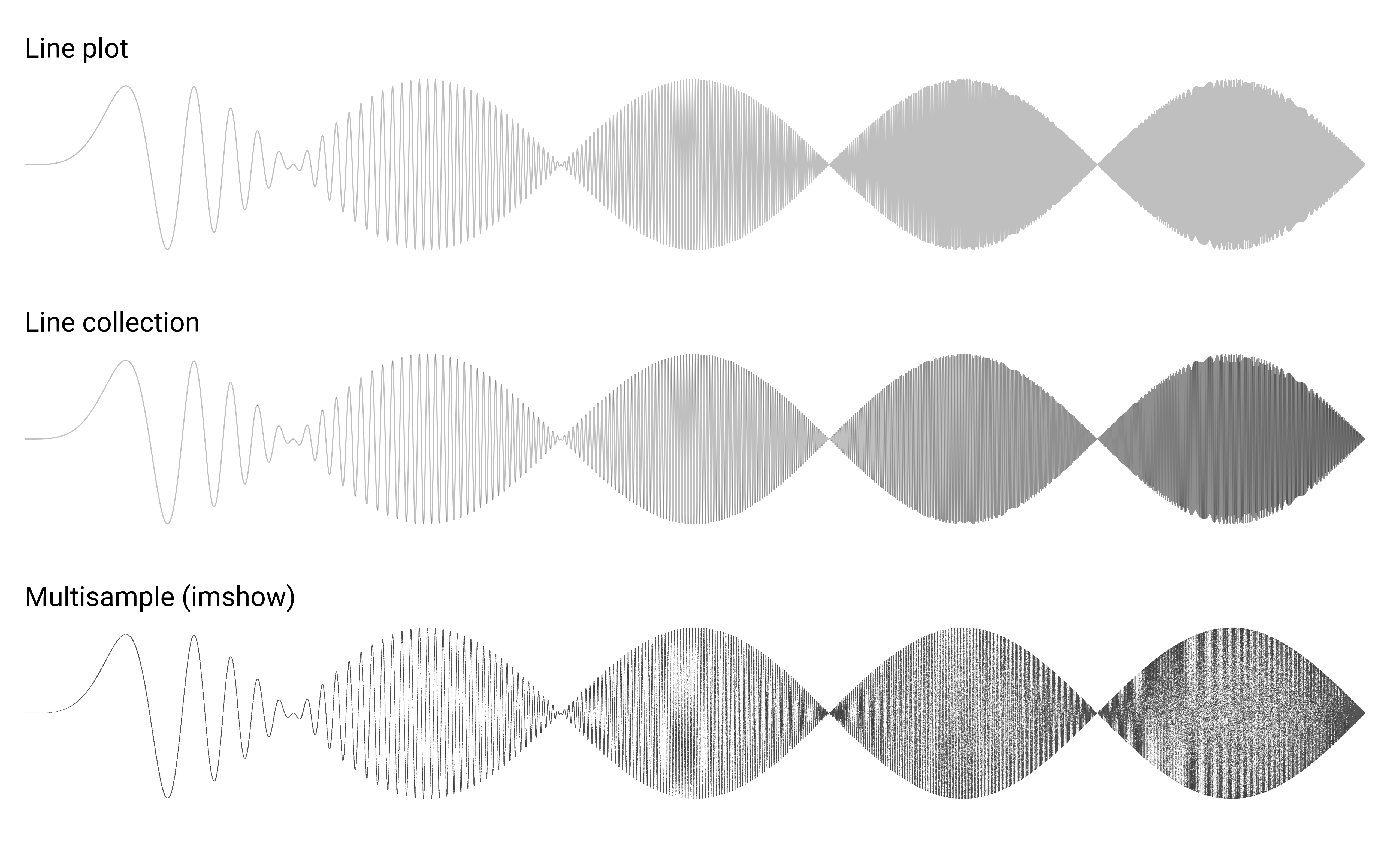
High-frequency signal. figure-multisample (sources: optimization/multisample.py).

Speed-up rendering

The overall speed of rendering a given figure depends on a number of matplotlib internal factors that are good to know. Even though the rendering speed is pretty decent in most cases, things can degrade very noticeably when you have a large number of objects and we’ve been already experienced such slowdown with the previous scatter plot examples. You may have noticed that there are two ways to render a scatter plot. Either you use the plot command with only markers or you use the dedicated scatter command. The two methods are similar and yet different. If you need a scatter plot where the size, shape and color of markers are the same, then you can use the plot command that is faster (by a factor of two approximately). For any other case, the scatter command is the one to use. We can try to measure the time to prepare a one million scatter plot using the following code:

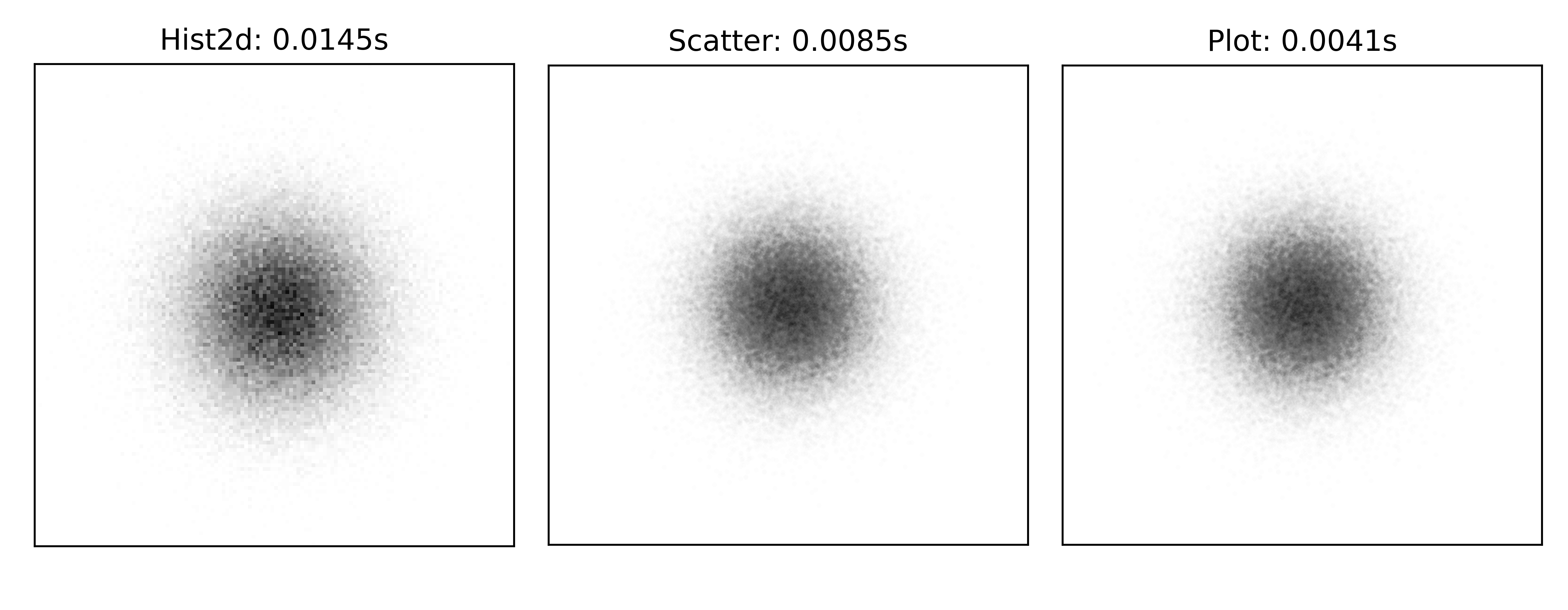
Scatter benchmark figure-scatter-benchmark (sources: optimization/scatter-benchmark.py).

By they way, you may have noticed the difference in size between plot (markersize=2) and scatter (s=2**2). The reason is that the size of marker in plot is measured in points while the size of markers in scatter is measured in squared points.

In the case of line plots, the difference in rendering speed between one solution or is the other can be dramatic as illustrated on figure figure-line-benchmark. In this example, I drew 1,000 line segments using 1,000 calls to the plot method (left), a single plot call (middle) with individual segment coordinates separated by None and a line collection (right). In this specific case, the choice of the rendering method makes a big difference such that for a large number of lines, your rendering can takes a few seconds or several minutes. Note that the fastest rendering (unified plot, middle) is not exactly equivalent to the others due to the absence of self-coverage as explained previously.

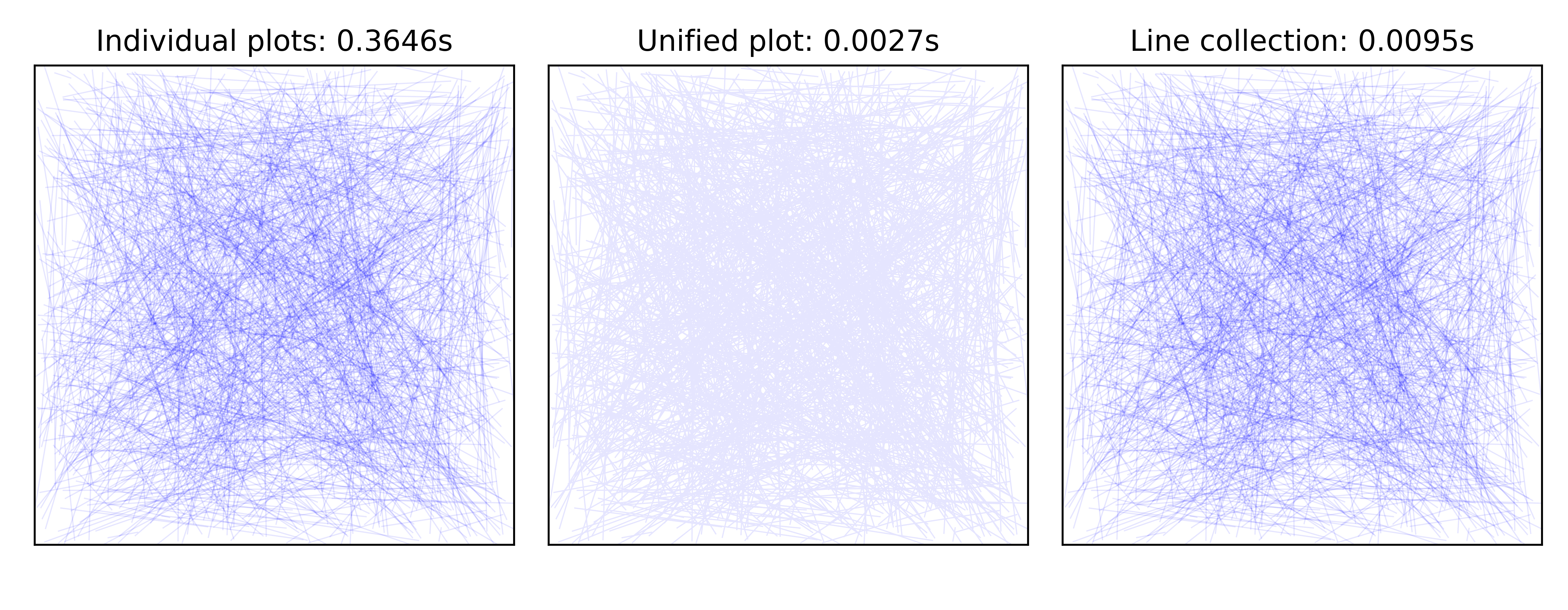
Line benchmark figure-line-benchmark (sources: optimization/line-benchmark.py).

File sizes

Depending on the format you save a figure, the resulting file can be relatively small but it can also be huge, up to several megabytes and this does not relate to the complexity of your script but rather to the amount of details or the number of elements. Let’s consider for example the following script:

plt.scatter(np.random.rand(int(1e6)), np.random.rand(int(1e6)))
plt.savefig("vector.pdf")

The resulting file size is approximately 15 megabytes. The reason for such a large file being the pdf format to be a vector format. This means that the coordinates of each point needs to be encoded. In our example, we have a million points and two float coordinates per points. If we consider a float to be represented by 4 bytes, we already need 8,000,000 bytes to store coordinates. If we now add individual color (4 bytes, RGBA ) and size (1 float, 4 bytes) we can easily reached 16 megabytes.

Let me now slightly modify the code:

plt.scatter(np.random.rand(int(1e6)), np.random.rand(int(1e6)),
            rasterized=True)
plt.savefig("vector.pdf", dpi=600)

The new file size is approximately 50 kilobytes and the quality is roughly equivalent even if it is not a pure vector format anymore. In fact, the rasterized keyword means that maplotlib will create a rasterized (i.e. bitmap) representation of the scatter plot saving a lot of memory when saved on disk. Incidentally, it will also make the rendering of your figure much faster because your pdf viewer does not need to render individual elements.

However, the combination of a vector format with rasterized elements is not always the best choice. For example, if you need to produce a huge figure (e.g. for a poster) with a very high definition, a pure vector format might be the best format provided you do not have too much elements. There’s no definitive recipes and the choice is mostly a matter of experience.

Multithread rendering

Multithread rendering is not natively supported by matplotlib but it is possible to do it anyway. The most obvious situation happens when you need to render several different plots. In such a case, there’s no real difficulty and it’s only matter of starting several threads concurrently. What is more interesting is to produce a single figure using multithread rendering. To do that, we need to split the figure into different and non overlapping parts such that each part can be rendered independently. Let’s consider, for example, a figure whose full extent is xlim=[0,9] and ylim=[0,9]. In such as case, we can define quit easily 9 non-overlapping parts:

X = np.random.normal(4.5, 2, 5_000_000)
Y = np.random.normal(4.5, 2, 5_000_000)

extents = [[x,x+3,y,y+3] for x in range(0,9,3)
                         for y in range(0,9,3)]

For each of these parts, we can plot an offline figure using a Figure Canvas and save the result in an image:

def plot(extent):

    xmin, xmax, ymin, ymax = extent
    fig = Figure(figsize=(2,2))
    canvas = FigureCanvas(fig)
    ax = fig.add_axes([0,0,1,1], frameon=False,
                      xlim = [xmin,xmax], xticks=[],
                      ylim = [ymin,ymax], yticks=[])
    epsilon = 0.1
    I = np.argwhere((X >= (xmin-epsilon)) &
                    (X <= (xmax+epsilon)) &
                    (Y >= (ymin-epsilon)) &
                    (Y <= (ymax+epsilon)))
    ax.scatter(X[I], Y[I], 3, clip_on=False,
        color="black", edgecolor="None", alpha=.0025)
    canvas.draw()
    return np.array(canvas.renderer.buffer_rgba())

Note that I took care of selecting X and Y that are inside the provided extent (modulo epsilon). This is quite important because we do not want to plot all the data in each subparts. Else, this would slow down things.

We can now put back every parts together using several imshow:

from multiprocessing import Pool

extents = [[x,x+3,y,y+3] for x in range(0,9,3)
                         for y in range(0,9,3)]
pool = Pool()
images = pool.map(plot, extents)
pool.close()

fig = plt.figure(figsize=(6,6))
ax = plt.subplot(xlim=[0,9], ylim=[0,9])
for img, extent in zip(images, extents):
    ax.imshow(img, extent=extent, interpolation="None")

plt.show()

If you look at the result on figure figure-multithread-rendering, you can observe a flawless montage of the different pieces. If you set the epsilon value to zero, you’ll observe white spaces appearing between the different parts. The reason is that if you enforce very strict clipping, a marker whose center is outside extent will not be drawn while it may overlap because of its size.

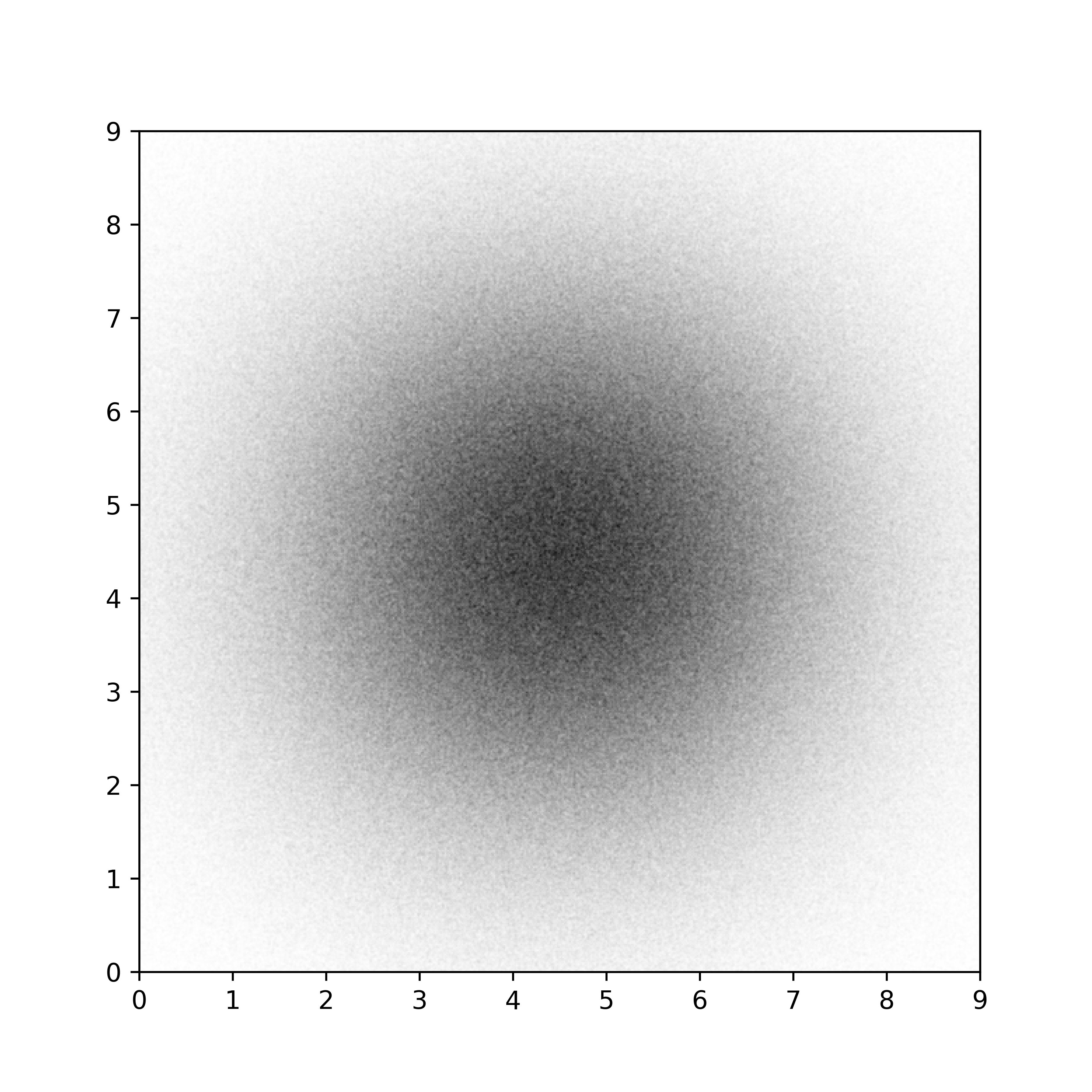
Multithread rendering figure-multithread-rendering (sources: optimization/multithread.py).

Such multithread rendering is not totally straightforward to implement because it depends on the possibility to split your in segregated elements. However, if you have a very complex plots that take several minutes to render, this is an option worth to be explored.