Graphic library

Beyond its usage for scientific visualization, matplotlib is also a comprehensive library for creating static, animated, and interactive visualizations in Python as written on the website. Said differently, matplotlib is a graphic library that can be used for virtually any purpose, even though the performance may vary greatly from one application to the other, depending on the complexity of the rendering. Such versatility can be explained by the presence of a number of low-level objects, that allow to produce virtually any rendering, and supported by a number of standard operations as shown on figure figure-polygon-clipping

Polygon clipping figure-polygon-clipping (sources: beyond/polygon-clipping.py).

Here is a first example showing the capability of matplotlib in terms of polygon and clipping. As you can see on figure figure-polygon-clipping, clipping allows to render any combination of two polygons.

Such clipping can be used as well in a regular figure to make some interesting effect as shown on figure figure-interactive-loupe.

Polygon clipping figure-interactive-loupe (sources: beyond/interactive-loupe.py).

Matplotlib dungeon

If you ever played role playing game (especially Dungeons & Dragons), you may have encountered “Dyson hatching” as shown on figure figure-matplotlib-dungeon (look at the outside border of the walls). This kind of hatching is quite unique and immediately identifies the plan as some kind of dungeon. This hatching has been originally designed by Dyson Logos who was kind enough to explain how he draws it (by hand). Question is then, how to reproduce it using matplotlib?

It’s actually not too difficult but it’s not totally straightforward either because we have to take care of several details to get a nice result. The starting point is a random two-dimensional distribution where points needs to be not too close to each other. To achieve such result, can use Bridson’s Algorithm which is a very popular method to produce such blue noise sample point distributions that guarantees that no two points are closer than a given distance. If you observe figure figure-bluenoise, you can see the algorithm makes a real difference when compared to either a pure uniform distribution or a regular grid with some normal jitters.

Uniform distribution, jittered grid and blue noise distribution figure-bluenoise (sources: beyond/bluenoise.py).

From this blue noise distribution, we can insert hatch pattern at each location with a random orientation. A hatch pattern is a set of n parallel lines with some noise:

def hatch(n=4, theta=None):
    theta = theta or np.random.uniform(0,np.pi)
    P = np.zeros((n,2,2))
    X = np.linspace(-0.5,+0.5,n,endpoint=True)
    P[:,0,1] = -0.5 + np.random.normal(0, 0.05, n)
    P[:,1,1] = +0.5 + np.random.normal(0, 0.05, n)
    P[:,1,0] = X + np.random.normal(0, 0.025, n)
    P[:,0,0] = X + np.random.normal(0, 0.025, n)
    c, s = np.cos(theta), np.sin(theta)
    Z = np.array([[ c, s],[-s, c]])
    return P @ Z.T

You can see the result in the center of figure figure-dyson-hatching. This starts to look like Dyson hatching but it is not yet satisfactory because hatches cover each others. To avoid that, we need to clip hatches using the corresponding voronoi cells. The easiest way to do that is to use the shapely library that provides methods to compute intersection with generic polygons. You can see the result on the right part of figure figure-dyson-hatching and it looks much nicer (in my honest opinion).

Dyson hatching figure-dyson-hatching (sources: beyond/dyson-hatching.py).

We are not done yet. Next part is to generate a dungeon. If you search for dungeon generator on the internet, you’ll find many generators, from the most basic ones to the much more complex. In my case, I simply designed the dungeon using inkscape and I extracted the coordinates of the walls from the svg file:

Walls = np.array([
    [1,1],[5,1],[5,3],[8,3],[8,2],[11,2],[11,5],[10,5],
    [10,6],[12,6],[12,8],[13,8],[13,10],[11,10],[11,12],
    [2,12],[2,10],[1,10],[1,7],[4,7],[4,10],[3,10],
    [3,11],[10,11],[10,10],[9,10],[9,8],[11,8],[11,7],
    [9,7],[9,5],[8,5],[8,4],[5,4],[5,6],[1,6], [1,1]])
walls = Polygon(Walls, closed=True, zorder=10,
                facecolor="white", edgecolor="None",
                lw=3, joinstyle="round")
ax.add_patch(walls)

The next step is to restrict the hatching to the vicinity of the walls. Since hatches corresponds to our initial point distribution, it is only a matter of filtering hatches whose centers are sufficiently close to any wall. It thus only requires to compute the distance of a point to a line segment. At this point, we do not care it the the hatch is inside or outside the dungeon since the internal hatches are hidden by the interior of the dungeon (see zorder above). I proceeded by adding dotted squares inside corridors using a collection of vertical and horizontal lines as well as some random “rocks” which are actually collection of small ellipses. Last, I added a nice title using an old looking font. I used Morris Roman font by Dieter Steffmann.

The result looks nice but it can be further improved. For example, we could introduce some noise in walls to suggest manual drawing, we could improve rocks by adding noise, etc. Matplotlib provides everything that is needed and the only limit is your imagination. If you’re curious on what could be achieved, make sure to have a look at one page dungeon by Oleg Dolya or the Fantasy map generator by Martin O’Leary.

Matplotlib dungeon figure-matplotlib-dungeon (sources: beyond/dungeon.py).

Tiny bot simulator

Using the same approach, it is possible to design a tiny bot simulator as shown on figure figure-tinybot which is a snapshot of the simulation. To design this simulator, I started by splitting the figure using gridspec as follows:

fig = plt.figure(figsize=(10,5), frameon=False)
G = GridSpec(8, 2, width_ratios=(1,2))
ax = plt.subplot( G[:,0], aspect=1, frameon=False)
...

for i in range(8): # 8 sensors
    sax = plt.subplot( G[i,1])
    ...

ax is the axes on the left showing the maze and the bot while sax are axes to display sensors value on the right. Maze walls are rendered using a line collection while the robot is rendered using a circle (for the body), a line (for the “head”, i.e. a line indicating direction) and a line collection for the sensors. The overall simulation is a matplotlib animation where the update function is responsible for updating the bot position and sensors values.

Tiny bot simulator figure-tinybot (sources: beyond/tinybot.py).

There is no real difficulty but the computation of sensors & wall intersection which can be vectorized using Numpy to make it fast:

def line_intersect(p1, p2, P3, P4):

    p1 = np.atleast_2d(p1)
    p2 = np.atleast_2d(p2)
    P3 = np.atleast_2d(P3)
    P4 = np.atleast_2d(P4)

    x1, y1 = p1[:,0], p1[:,1]
    x2, y2 = p2[:,0], p2[:,1]
    X3, Y3 = P3[:,0], P3[:,1]
    X4, Y4 = P4[:,0], P4[:,1]

    D = (Y4-Y3)*(x2-x1) - (X4-X3)*(y2-y1)

    # Colinearity test
    C = (D != 0)
    UA = ((X4-X3)*(y1-Y3) - (Y4-Y3)*(x1-X3))
    UA = np.divide(UA, D, where=C)
    UB = ((x2-x1)*(y1-Y3) - (y2-y1)*(x1-X3))
    UB = np.divide(UB, D, where=C)

    # Test if intersections are inside each segment
    C = C * (UA > 0) * (UA < 1) * (UB > 0) * (UB < 1)

    X = np.where(C, x1 + UA*(x2-x1), np.inf)
    Y = np.where(C, y1 + UA*(y2-y1), np.inf)
    return np.stack([X,Y],axis=1)

This simulator could be easily extended with a camera showing the environment in 3D using the renderer I introduced in chapter `chap-3D`_. In the end, it is possible to write a complete simulator in a few lines of Python. The goal is of course not to replace a real simulator, but it comes handy to rapidly prototype an idea which is exactly what I did to study decision making using the reservoir computing paradigm.

Real example

When put together, these graphical primitives allow to draw quite elaborated figures as shown on figure figure-basal-ganglia. This figure comes from the article A graphical, scalable and intuitive method for the placement and the connection of biological cells that introduces a graphical method originating from the computer graphics domain that is used for the arbitrary placement of cells over a two-dimensional manifold. The figure represents a schematic slice of the basal ganglia (striatum and globus pallidus) that has been split in four different subfigures:

• Subfigure A is made of a bitmap image showing an arbitrary density of neurons. I used a bitmap image because it is not yet possible to render such arbitrary gradient using matplotlib. However, I also read the corresponding SVG image to extract the paths delimiting each structure and plot them on the figure.

• Subfigure B represents the actual method for positioning an arbitrary number of neurons enforcing the density represented by the color gradient. To represent them, I used a simple scatter plot and colored some neurons according to their input/output status.

• Subfigure C represents an interpolation of the activity of the neurons and has been made using a 2D histogram mode. To do that, I simply built a big array representing the whole image and I set the activity around the neuron using a disc of constant radius. This is only a matter of translating the 2d coordinates of the neuron to a 2D index inside the image array. I then used an imshow to show the result and I drew over the frontiers of each structure. This kind of rendering helps to see the overall activity inside the structure.

• Subfigure D is probably the most complex because it involved the computation of Voronoi cells and their intersection with the border of the structure. Once again, the shapely library is incredibly useful to achieve such result. Once the cell have been computed, it is only a matter of painting them with a colormap according to their activity. For efficiency, this is made using a poly collection.

This is actually quite a complex example, but once you’ve written the code, it can be adapted to any input (the SVG file in this case) such that your final result is fully automated. Of course, the amount of work this represents should be balanced with your actual needs. If you need the figure only once, it is probably not worth the effort if you can do it manually.

A schematic view of a slice of the basal ganglia. Sources availables from the spatial-computation repository on GitHub. figure-basal-ganglia

Exercises

Stamp like effect Fancy boxes offer several style that can be used to achieve different effect as shown on figure figure-mona-lisa-stamp. The goal is to achieve the same effect.

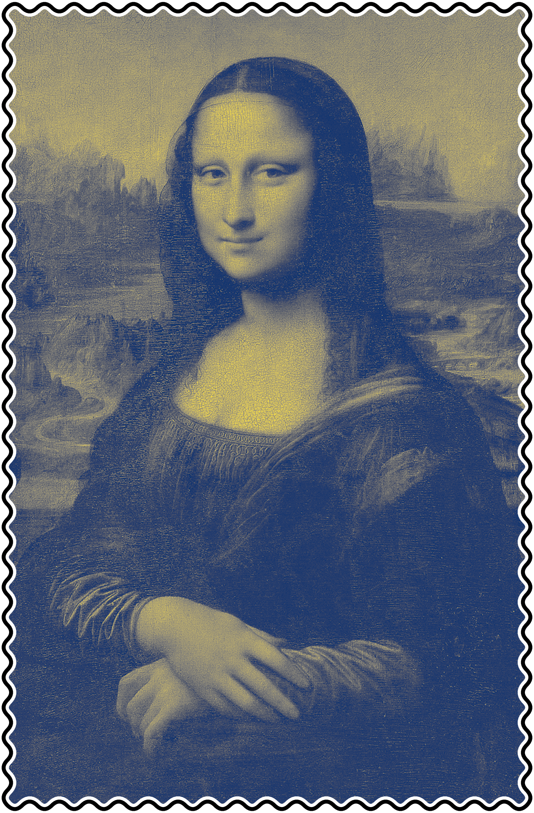
Mona Lisa stamp figure-mona-lisa-stamp (sources: beyond/stamp.py).

Radial Maze Try to redo the figure figure-radial-maze which displays a radial maze (that is used quite often in neuroscience to study mouse or rat behavior) and a simulated path representing a rat exploring the maze (this has been generated by recording the (computer) mouse movements). The color of each block represents the occupancy rate, that is, the number of recorded point inside the block.

Radial maze figure-radial-maze (sources: beyond/radial-maze.py).